Introduction
This project uses data collected from lake sediment samples to reconstruct past changes in the environment. The focus of the current work is on reconstruction of Total Phosphorus. Sediment Core samples were collected from two Minnesota lakes. Layers of each core were then separated for further study. Fossil remains of Diatoms were counted and identified using a microscope. Diatoms are single celled algae that are abundant in lakes and leave behind an identifiable cell wall in sediments. There are many Diatom species and their community makeup can be used to reconstruct past environmental conditions. Also, a depth in the core can be dated to a past time period.
Description of Data
Ecologists collected a core sample from the two lakes. The data consists of counts of diatoms at the genus level for multiple depths of each core sample. A diatom calibration set and corresponding Environmental data set was used (Edlund and Ramstack 2006). The full calibration set consists of 155 samples with relative abundance of 759 diatom species in sediment samples from Minnesota lakes. The environmental data set has measurements of Total Phosphorus in each of the 155 samples. The calibration data set identified diatoms at a species level. However, the data only identified diatoms at the genus level. A limnologist selected species codes from the calibration set to replace the genus identification.
Edlund and Ramstack (2006) give criteria of keeping diatom species if they have greater than 1% relative abundance in two or more samples, or greater than 5% relative abundance in one sample. Based on this criteria, diatoms identified with genus Nitzchia in Lake 1, and genus Cymbella, Cavinula and Acanthocerus in the Lake 2 could have been kept for analysis. Since they were not identified by collaborator, they were removed. For the calibration data set, the Edlund and Ramstack criteria were applied. However, this removed species identified in the data set, so they were added back. Species codes ACHEXILI, MELVARIA, CAVJAERN, and ACOZACHA would be removed by criteria, but were kept because of their abundance in the collected data. As an example, MELVARIA had the highest relative abundance in the data set, but only accounts for 1.79 % of Diatoms in the calibration set.
Edlund and Ramstack (2006) identified the lakes Dickman, George in Blue Earth Co., and Loon in Jackson Co. as outliers in the data set. These samples were removed. Based on the criteria for using diatoms and outliers, the final data set had 164 diatom species and 152 samples. To make the data usable by our tools for Statistical Analysis, the count data was converted to relative abundance. Both the Calibration and collected diatom set were transposed to have diatom names as columns and sample identification in rows.
Statistical Analysis
Methods
The distribution of species among samples was originally explored using canonical correspondence analysis (CCA). CCA is a multivariate method that works to explain the relationship between a collection of biological species and their environment. Some of the variables used in this method were transformed using \(log_{10}\) to meet the condition of normality. The variables included in the model are: log(Total Phosphorus), log(Max Depth), pH, log(Color), log(Chloride), and Conductivity. These six variables were used because they were found to show significant variation in the species data in the article by Edlund and Ramstack (2006). The CCA method is used to identify the variables that independently explain a significant portion of the variance in the species data.
Following the CCA, Weighted Averaging regression was used to build a model of environmental variables based on a calibration data set (Edlund and Ramstack 2009). Weighted averaging regression generates a transfer function with diatom assemblages and environmental measures like Total Phosphorus. The environment determines composition of diatom species. In the transfer function, we model the reverse of the relationship. We model diatoms inferring environmental variables. Diatoms do not cause changes in Total Phosphorus levels, but using diatoms as predictors allows us to reconstruct past environmental conditions. The data comes from modern sediment samples where it is possible to measure total phosphorus. Diatoms are identified in a sample to connect relative abundance of species to environment.
In weighted averaging, the diatom relative abundance are used as the predictors and Total Phosphorus used as response. The weighted averaging takes multiple averages, which shrinks the range of estimates. A deshrinking step is applied on the results of Weighted Averaging to correct the narrowed range.
Results
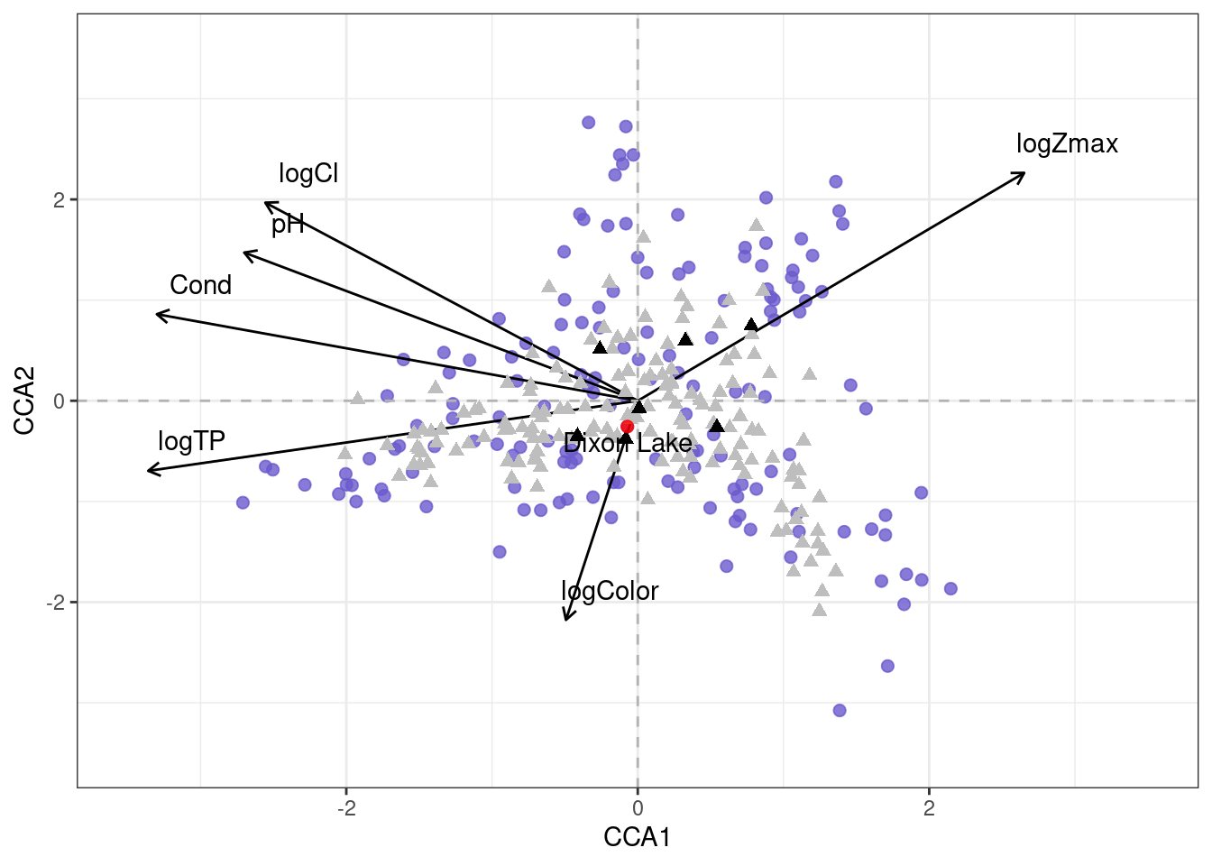
The results of the CCA show that the 6 environmental variables explain 16.26% of the variation in species data with 5.4% and 3.5% of the variation explained by axis 1 and 2, respectively. The significance of each variable was tested independently (\(p\) \(\leq\) \(0.05\)). It was found that Total Phosphorus was the most explanatory variable, accounting for 4.7% of the total variation in species data. Each of the other five environmental variables were significant as well, and the percent of variance explained by each is: Max Depth (2.8%), pH (2.7%), Color (1.9%), Chloride (1.8%), and Conductivity (2.45%).
A CCA biplot of the environmental variables show some correlations between the variables and the axis (Figure 1). We can see that log(Total Phosphorus) and Conductivity are correlated with axis 1, while log(Color) is correlated with axis 2. Another interpretation of Figure 1 is that Lakes plotted near each other have similar assemblages, and by reconstruction similar environmental conditions. Dixon Lake, which is nearby both the lakes, is plotted for reference. Also, the species that were identified in both the lakes from the collected data are shown as black triangles (Figure 1).
Figure 2 compares the predicted Weighted Averaging log TP to the actual log TP. Having a random scatter and visibly linear trend around a line with slope 1 and intercept 0 shows the model predicts the training set well.
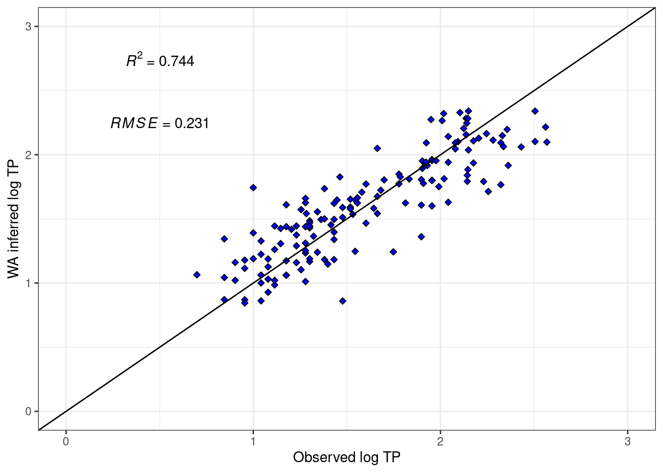
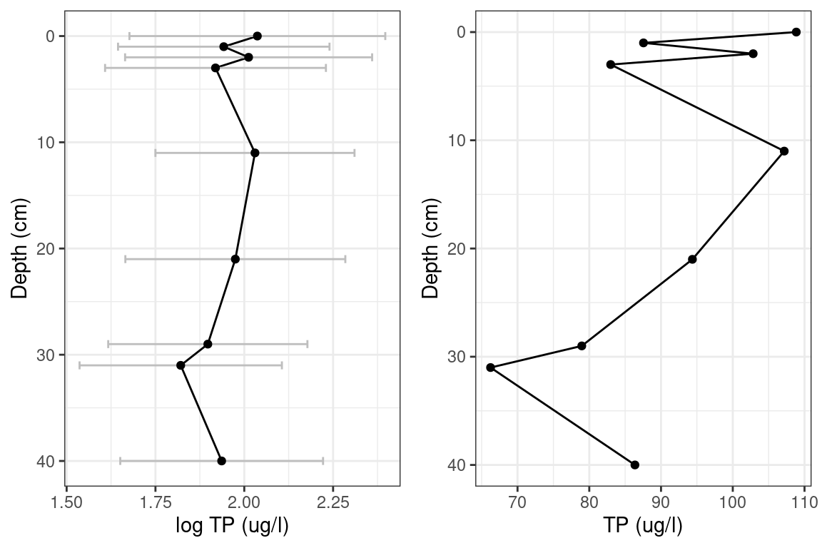
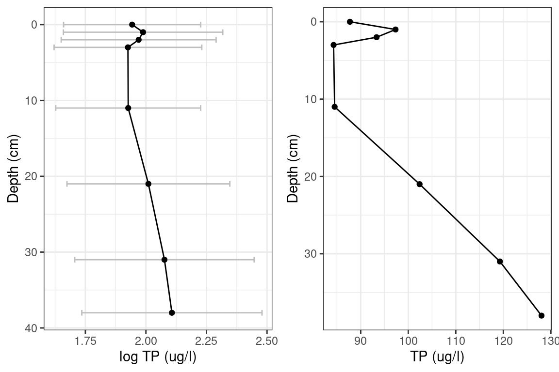
Figure 3 and 4 show reconstructed log TP for Lake 1 and Lake 2. The log TP plots have error bands of Root Mean Squared Error of Prediction. This is analogous to one Standard Deviation from the mean.
A report for Lake 1 from 2015 showed a total phosphorus range between 21 ug/L and 88 ug/L with a mean of 45.2 ug/L. Converted to \(log_{10}\) gives a mean of 1.66, and range between 1.32 and 1.94. The Lake 1 model predicts a range in 2019 of 1.61 to 2.23 with mean 1.92. The log of the mean of the 2015 Lake 1 total phosphorus falls within one standard deviation of the model prediction.
A report for Lake 2 from 2007 showed a total phosphorus range between 26 ug/L and 85 ug/L with a mean of 44 ug/L. Converted to \(log_{10}\) gives a mean of 1.64, and range between 1.41 and 1.92. The Lake 2 model predicts a range in 2011 as 1.63 to 2.23 with mean 1.93. The log of the mean of the 2006 Lake 2 total phosphorus falls within one standard deviation of the model prediction.
Conclusion
Measuring historical total phosphorus levels is often not possible. An alternative is to use diatom relative abundances to reconstruct historical environmental conditions. Diatoms are strongly influenced by environmental conditions, and can be used to reconstruct total phosphorus, for example.
From the CCA with 6 environmental variables, we found that \(log_{10}\) of Total Phosphorus explained the most variation in species data. Weighted averaging with inverse deshrinking was used to predict \(log_{10}\) of Total Phosphorus with Diatom abundances as the predictors. Past water quality reports of both Lakes were referenced for modern actual total phosphorus. The \(log_{10}\) of the actual mean was within one standard deviation of the predicted \(log_{10}\) of Total Phosphorus for both Lakes.
Future work could include using different methods for transfer function. Do sampling similar to (Edlund and Ramstack 2009). They had a minimum of 400 diatoms counted per sample. Diatoms were identified at species level in the calibration set, whereas new data was identified at genus level. Identification at species level and higher diatom counts per sample could improve model accuracy. Use of the criteria of 1% relative abundance in two or more samples, or 5% in one sample could give more species for prediction. Identifying the original 89 lakes used in Edlund and Ramstack model would help for reproducibility of their original results for the CCA analysis and Weighted Averaging model. The current work used 152 samples from Edlund and Ramstack dataset. Sites are identified by codes. Having an easy way to translate site codes to lake names would be useful in identifying sites.
References
Edlund, M, and J. Ramstack. 2006. Science Museum of Minnesota: Diatom-Inferred TP in MCWD Lakes. Available at: https://www.minnehahacreek.org/sites/minnehahacreek.org/files/attachments/MCWDFinalRpt06_07.pdf
Edlund, M, and J. Ramstack. 2009. Science Museum of Minnesota: Historical Water Quality and Biological Change in Northcentral Minnesota Lakes. Available at: https://www.smm.org/sites/default/files/public/attachments/2009_edlund._historical.pdf
Simpson, G.L. and J. Oksanen. 2021. analogue: Analogue matching and Modern Analogue Technique transfer function models. (R package version 0.17-6 ). (https://cran.r-project.org/package=analogue)
Simpson, G.L. (2007). Analogue Methods in Palaeoecology: Using the analogue Package Journal of Statistical Software, 22(2), 1–29
Oksanen, J. F. Guillaume Blanchet, M. Friendly, R. Kindt, P. Legendre, D. McGlinn, P.R. Minchin, R.B. O’Hara, G.L. Simpson, P. Solymos, M. Henry H. Stevens, E. Szoecs and H. Wagner. 2020. vegan: Community Ecology Package. R package version 2.5-7. https://CRAN.R-project.org/package=vegan
Oksanen, J. 2020. Vegan: an introduction to ordination. Available at: https://cran.r-project.org/web/packages/vegan/vignettes/intro-vegan.pdf
Adler, S. and Hübener, T. 2018. R for palaeolimnology – a manual. Avaiblable at: https://www.botanik.uni-rostock.de/storages/uni-rostock/Alle_MNF/Bio_Botanik/R-for-palaeolimnology-version_09-12.pdf
Lake Names. Minnesota Conservation Department. Available at: http://files.dnr.state.mn.us/publications/waters/LAKENAMES_BULL25.pdf
Vegan cheat sheet. RPubs. (n.d.). Available at: https://rpubs.com/an-bui/vegan-cheat-sheet
Dixon Lake Itasca County (n.d.). Available at: https://www.rmbel.info/wp-content/uploads/2017/11/Dixon-Lake-31-0921-00.pdf